Introduction
The goal of this project is to identify the time of onset or wakeup event based on wrist worn accelerometer data. This project was taken up from Kaggle1.
To this end, we are given roughly 300 continuous series of accelerometer data, with each series corresponding to a single wrist-worn accelerometer’s data collected over a long period of time2. Each series of data contains the following information:
- An ID for the series.
- Timesteps.
- Timestamps corresponding to the datetime in ISO 8601 format.
- The z-angle of the accelerometer, giving the relative position of the arm to the vertical axis of the body.
- The ENMO (Euclidean Norm Minus One) of all accelerometer signals.
We are also given a CSV file which is the translation of this data into sleep logs3, which for each series is translated into the following data:
- An ID for the series.
- Groups of timesteps are compiled into “Nighttime,” which determines when a sleep occurrence can happen.
- Events - either an “Onset” or a “Wakeup.”
- The step/timestamp of each event.
The data is subject to certain parameters; “Onset” and “Wakeup” mark the beginning and end of a sleep occurrence. These can only occur during “Nighttime.” Only one sleep occurrence can occur during a single “Nighttime”. To classify as a sleep occurrence, the beginning and end must be more than 30 minutes apart and cannot be interrupted by a period of time longer than 30 minutes. If there are multiple sleep occurrences in a night, only the longest one is recorded.
Each data series also contains periods of time where the accelerometer is removed from the wrist and stays completely still - these periods must be free of events.
The actual problem involves roughly 200 continuous series of accelerometer data similar to the data given4 - however, there is no accompanying CSV file translating the data into sleep logs. Rather, we must create a model that trains using the original data and its corresponding sleep logs and can then predict when events will take place throughout a new series of accelerometer data, with each event being given a confidence score. This data should then be usable to create a corresponding sleep log.
The entire project is hosted on GitLab5. The final prepared datasets and trained models are copied and provided in the drive6.
Methodology
Data Preparation
-
Selected windows around events: We hypothesize that an onset of wake or sleep is mostly tied to changes in the observation data rather than the exact values of the data themselves. Thus, we extend the naive event structure to include a window of observation time steps both before and after the event, capturing the context that the event occurred in. These “windows” will be labeled according to the event that they are centered around.[7] We take an interval of 30 steps around the event to predict the event itself.
-
Sliding window: We also include data for time steps in which no event occurs by building windows of observation for every time step in the observation sequence. Our data setup now looks like a sliding window of observations taken from each observation sequence in the given data, with each window instance being labeled according to the event located in the center of the interval. It’s important to note that some time steps in the observation sequence have missing data, so we are careful to skip over these “null” steps when constructing our observation windows.[8]
-
Gaussian Kernel window: To increase the feature space of our dataset and provide more information regarding the sleep states, we introduce a gaussian kernel distribution to represent the probability of an event. This idea is based out of keypoint regression or heatmap detection problems9.
We consider hour-long windows (each step is 5 seconds apart, making each hour combination of 720 rows). For each hourly window, based on the time when the
onsetorwakeupevent occurs, we sample points from a normal distribution for both the events. Thus, the output becomes 720 x 2 datapoints that represent the probabilities ofonsetandwakeup. The input variables are the list ofanglezandenmo. Both the output and input variables are sorted by time.Since this dataset preparation was a larger task, we split it up into two parts:
- Supplement the series dataset with probabilities of event happening sampled from normal distributions using kernel density, taking the mean to be the actual occurrence of the event[10].
- Grouping this supplemented dataset by hour[11].
These probabilities are paired with the anglez and enmo values. Splitting up our data by hour long intervals also allows the RNN to account for how the sleep and wake events change over a longer time.
Model Selection
-
RNN
Considering that our data set is a series, the first immediate choice for a model was a recurrent neural network (RNN). A RNN is a form of an artificial neural network, where the outputs can influence subsequent inputs. This allows for advanced pattern recognition, especially in problems that involve a sequence or a time-step. We specifically use a Long short-term memory model (LSTM). Our network contains a bi-directional layer followed by two fully connected layers. The bidirectional LSTM layer takes in 2 features for an input and has 128 features as the output. The fully connected layer takes in 256 features from the LSTM layer, and outputs 50 features after RELU activation to the fully connected output layer. The output layer produces 1 feature after sigmoid activation, giving the probability of an event being sleep or wake event.12 We consider this model for both selected windows around events and sliding window and labels technique.
CustomModel( (lstm): BidirectionalLSTM( (lstm): LSTM(2, 128, batch_first=True, bidirectional=True) ) (fc1): Linear(in_features=256, out_features=50, bias=True) (relu): ReLU() (fc2): Linear(in_features=50, out_features=1, bias=True) (sigmoid): Sigmoid() ) -
Gaussian Kernel with RNN
We modify our RNN to work with our Gaussian Kernel window data and predict the probability of on-set and wake for a given anglez and enmo value. We considered two different models in this approach. One was bounded by sigmoid in the last layer (Model A) whereas the other was not (Model B). The basic ideas was to scale the targets (probabilities) to have a higher loss for making wrong predictions on probabilities which are non zero vs having a sigmoid layer in the end and not scaling up the target probabilities. Except the last layer we follow a similar RNN structure previously mentioned. However, our bi-directional LSTM layers now outputs a hidden size of 2x2048. The fully connected layer takes in 4096 features and outputs 2048 features to the output layer using a RELU activation function. The fully connected output layer provides 720*2 outputs representing probability of sleep and wake respectively. These two models has significantly more parameters to train compared to our baseline RNN model.13
CustomModel( (lstm): BidirectionalLSTM( (lstm): LSTM(2, 2048, batch_first=True, bidirectional=True) ) (fc1): Linear(in_features=4096, out_features=2048, bias=True) (relu): ReLU() (fc2): Linear(in_features=2048, out_features=1440, bias=True) (sigmoid): Sigmoid() )CustomModel( (lstm): BidirectionalLSTM( (lstm): LSTM(2, 2048, batch_first=True, bidirectional=True) ) (fc1): Linear(in_features=4096, out_features=2048, bias=True) (relu): ReLU() (fc2): Linear(in_features=2048, out_features=1440, bias=True) (relu2): ReLU() ) -
SVM
To evaluate the performance of a more classical machine learning method, we choose to train a purely linear support vector machine that uses no kernel embedding of the data. Since support vector machines cannot take the sequential nature of our data into account, we will simply flatten out our windows of observation into long one-dimensional vectors. Even though the SVM may not fully take advantage of the context of the observations it is given, perhaps the higher dimensionality granted by the additional observations within the window may still allow the SVM to learn a somewhat sophisticated relationship between the observations and the events.[14]
Training
Selected windows around events and Sliding window
We train our RNN model on the entire dataset with a sliding window of 30 steps for both Selected windows around events and Sliding window approaches[15]. To increase the speed of training, we use distributed computing using Torch and Ray which is explored more in resource allocation. Our model has 14075 trainable parameters. We use a train-test split of 0.25 with 10 epochs. The learning rate is 0.01 and the batch size used is 32. We use a mean-squared error loss and stochastic gradient descent for optimization. We use ray to keep track of the training process and report the loss. The latest model is saved and used for inference.
Gaussian Kernel with RNN
We train both the models (Model A and Model B) mentioned in the above section for this approach on the prepared dataset after grouping the data (as mentioned in reference [11]) using PyTorch in Ray[16]. We use a batch size of 32 and with 5 epochs of training data and save the model after each epoch for reinstantiating from the same checkpoint in case of training failure (since this was being done on a large dataset). As mentioned, this model was taking very long time in training due to large parameters. The logfile for training has been referenced17. We observed that the loss decreased exponentially with each epoch generally but increased slightly at 4th.
Resource Allocation
We extensively make use of two services:
- Dataproc18 by Google: Dataproc is a cloud-based, fully managed service provided by Google Cloud Platform (GCP) for processing and analyzing large datasets using popular open-source frameworks such as Apache Hadoop, Apache Spark, Apache Hive, Apache HBase, and more. We use it only for Apache Spark for transforming the large dataset in all our scripts. The basic appraoch has been to perform a good enough analysis and transformation on jupyter notebook locally and run the same script by download it as a python file on Dataproc cluster. The inputs and outputs of each job are paths to Cloud Storage service by Google Cloud where we save the data in buckets. The next process is to manually download it and move it for training and inference to the respective machine.
- Ray19: Ray is an open-source distributed computing framework primarily designed for high-performance and scalable parallel and distributed Python applications. It is developed by the RISELab at UC Berkeley. Ray Train distributes model training compute to individual worker processes across the cluster. Each worker is a process that executes the
train_func. The number of workers determines the parallelism of the training job and is configured in theScalingConfig.
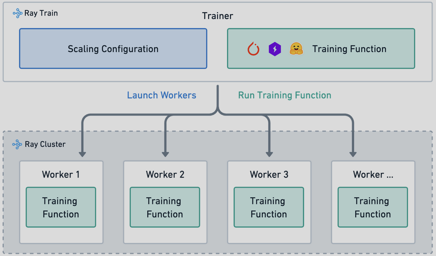
Ray Training Architecture
We managed Dataproc access through free credits on joining Google Cloud and sharing the access to sleep detection project to different team members using IAM policies and service accounts. Moreover, since ray acts as a service on a cluster, we used the on campus cuda cluster which had 5 nodes and 16GB GPUs on each node to train our dataset. Ray also managed scheduling jobs for the entire team as the resources were becoming free so helped us work in parallel.
Experiments & Result Analysis
RNN
Selected windows around events
We observe a validation accuracy of 67.42%. This naive approach converges on the test dataset and we get an accuracy of 67.03%20. Since this was the first naive approach, we skipped creating the confusion matrix for it.
Sliding window
We use a subset of our data for inference and analysis. We use a batch size of 5 during inference. To classify events as sleep or wake, we take any value above 0.5 from our sigmoid output as sleep, else wake. Using the Sklearn library, we create a confusion matrix to see the accuracy in our classification of events as sleep or wake. We observe an average test accuracy of 88.1% for 50,000 events[21].

Confusion Matrix for test dataset using RNN (sliding window)
We take our analysis a step further to identify the accuracy in the time of prediction - i.e., is our model able to accurately predict when sleep states change into wake. These changes of events are on-set (sleep to wake) and wake-up (wake to sleep). If on-set or wake-up are predicted within 5 seconds of the change in events in the ground truth data, we classify it as a true positive event. Else, the predicted change in event is a false positive.
| True Positive | 1830 |
|---|---|
| False Positive | 767404 |
| Total Predicted Events | 769234 |
| Total Events in Ground Truth | 7202 |
If we disregard false positive events, the predicted events have an accuracy of 25%. The excess number of predicted events can occur due to the accuracy of 88% during classification. This often means that 10-12% of the data is misclassified, which leads to incorrect predictions around those misclassifications.
Gaussian Kernel with RNN
For inference on Gaussian Kernel, we created a threshold of 0.2 and any step which crossed this value was considered as an onset or wakeup event. We perform a naive inference to test the accuracy of our model. For probabilities above our threshold, we check for change in sleep-state events. If these match, we count the event as a true positive, else it is a false positive event. The probabilities output from the model overall matches the pattern in sleep-states. We observe an accuracy of 20% (out of predicted timestep, 20% were actual timest) between all our hyperparameter tuning, however we do not believe that this represents the model’s true capabilities as due to time constraints our model was trained on a very small sample size for 5 epochs only. However, our probabilities were highly descriptive on the sleep-state events. For example, a change in probability by 20% is enough to predict an event. We believe that finding the right hyperparameter can significantly increase the accuracy of our model22.
SVM
For training the linear support vector machine, we elect to use a subset of the full data due to the space constraints of storing and fitting to the data. Additionally, we only consider two labels: no change, and wake onset, so we will only need to fit a single binary SVM. We utilize an observation window length of 30 (that is, 15 observations ahead and 15 behind the central time step), and flatten the entire window into a long one-dimensional vector that will be fed into the SVM during training. Due to the size of the data set we are fitting to, we trained the SVM using stochastic gradient descent, letting the training process run for 5 epochs with a batch size of 2048. To normalize the data, we calculate mean and standard deviation for the whole training set, and then normalize each batch accordingly while we perform gradient descent. Our test data is also normalized by these same training statistics to allow performance to be independent of batch size during test time. Our trained SVM achieved an accuracy rate of around 56.59%, and the resulting confusion matrix can be seen below:

Confusion Matrix for SVM Approach
where 0 represents “no change” and 1 represents “wake”. While the classifier does perform better than random, it obviously still has a long way to go in order to achieve an acceptably high success rate (barring the omission of the third label). However, we observe the SVM’s ability to avoid overfitting to the “no change” label, even if it is present in a much higher proportion in the training data.
Future Work
After analysing the results from our models, we explored other approaches from the various submissions made to this Kaggle competition which ended on December 5th. We have found multiple avenues from which we can improve the performance of our models.
One general improvement to our work is improving the inference and analysis of our models to truly understand which model performs better for this task. Specifically, the Gaussian RNN model which required finding the right threshold and plenty of training. We may also consider more features or layers as this model is the most descriptive on the peaks of our data.
- We can consider increasing our feature space to include more than anglez and enmo. This would also require improving our model to account for these additional features. Some common approaches we see are the use of convolutional neural networks such as a U-Net (statistical measures like mean/variance of anglez and enmo as input to these models).
- We can also try out a pretrained NN in place of training an RNN from scratch in different approaches.
- We can consider approaches used in academic papers and research in sleep state detection. Some of the more popular approaches are Random Forests and vanHees Approach [23].
References
[10]: https://gitlab.com/math5465/sleep-detection/-/blob/main/DataTransformation/Transformation Gaussial Kernel.ipynb?ref_type=heads, corresponding Dataproc script: https://gitlab.com/math5465/sleep-detection/-/blob/main/dataproc/transform_gaussian.py?ref_type=heads, output directory in bucket: gaussian_kernel
[11]: https://gitlab.com/math5465/sleep-detection/-/blob/main/DataTransformation/Group.ipynb?ref_type=heads, corresponding Dataproc script: https://gitlab.com/math5465/sleep-detection/-/blob/main/dataproc/group.py?ref_type=heads, output directory in bucket: group_sorted
[14] https://gitlab.com/math5465/sleep-detection/-/blob/main/SVM/SVM.ipynb?ref_type=heads
[15]: https://gitlab.com/math5465/sleep-detection/-/blob/main/RNN/training.py?ref_type=heads, example script: ray job submit --no-wait --working-dir . -- python [training.py](http://training.py/) --data '/home/prabhjot/data_frame_30/' -e 10 -g True -w 2
[16]: https://gitlab.com/math5465/sleep-detection/-/blob/main/RNN/training_gaussian.py?ref_type=heads, example script: ray job submit --no-wait --working-dir . -- python training_gaussian.py --data '/project/rl-umn/group_all_sorted' -e 5 -g True -w 3 -b 32
[23]: Sundararajan, K., Georgievska, S., te Lindert, B.H.W. et al. Sleep classification from wrist-worn accelerometer data using random forests. Sci Rep 11, 24 (2021). https://doi.org/10.1038/s41598-020-79217-x